Related Posts
Ways to fix VALUE error in Excel 2016

Written By
Sahil Verma
Updated On
August 28, 2025
Read time 6 minutes
While using Microsoft Excel 2016, you must have encountered #VALUES error. This error appears when you enter a wrong value in the function or formulas. It is Excel’s way of telling you that there’s a problem with the type of data being used in a formula or function.
The regular addition and subtraction operation with a (+) or minus (-) operator will throw a #VALUE! error if any of the values is not of the expected type. However, the #VALUE! error for some functions is a bit tricky because they automatically ignore the invalid data.
Let us consider some of the most common examples of #VALUE! error along with the solutions to resolve them.
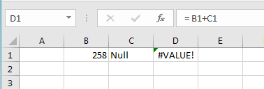
Consider the example below, where the Cell C2 contains a text value ‘Null’ while Cell B1 contains a numeric value ‘258’. When formulated “= C1 + B1”, D1 returns the #VALUE! error.
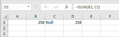
One standard solution for this is to correct the invalid value. However, while working with large spreadsheets, correcting individual data will consume a lot of time and efforts. In that case, we will use the SUM function to get rid of the #VALUE! error.
However, the SUM function ignores the invalid value as shown below:
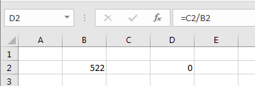
Consider the example below, where C2 cell is left blank, and cell B2 contains a numeric value (522). When formulated “=C2/B2”, D2 returns a #DIV/0! error, which indicates division by zero.
Now, if the same cell C2 contains errant space characters, D2 will throw a #VALUE! error.
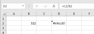
Users can look out for errant space characters by pressing the F2 key within the cell to note the blinking cursor, as shown in the image below.
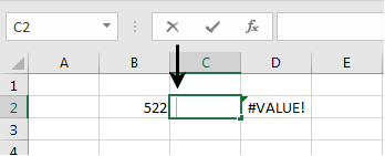
If the cursor seems to be a couple of millimeters away from the adjacent border of the cell, press the Delete key.
However, while working on large spreadsheets, you can use the ISBLANK function to determine whether a cell is blank or not. The function will return TRUE if the cell is blank or FALSE if it’s not.
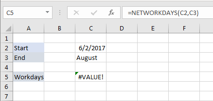
dates. If one of the function arguments is not the expected type, Excel will throw a #VALUE! Error.
In the example below, cell C2 contains the start date (6/2/2017), and cell C3 contains an invalid value “August.” As a consequent, cell C5 returns #VALUE! Error.
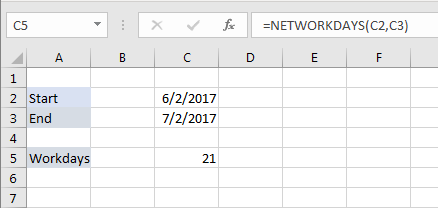
Enter the correct value as a date to get the desired result.
When you work on large spreadsheets, you may face Excel corruption issues in addition to issues like #VALUE! Error. Though there are some manual ways to Recover Corrupted Excel 2016 files, try to use a trusted third-party tool to fix your Excel error codes as manual Excel recovery methods are time-consuming and complicated.
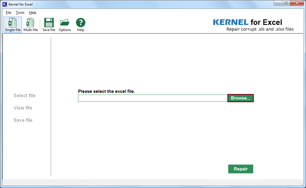
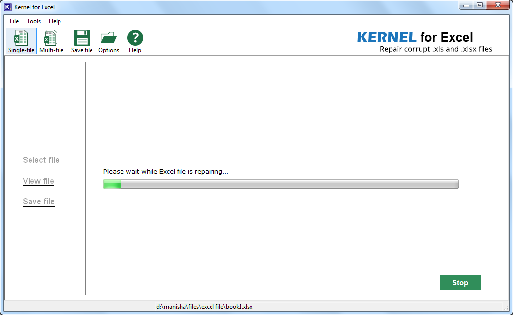
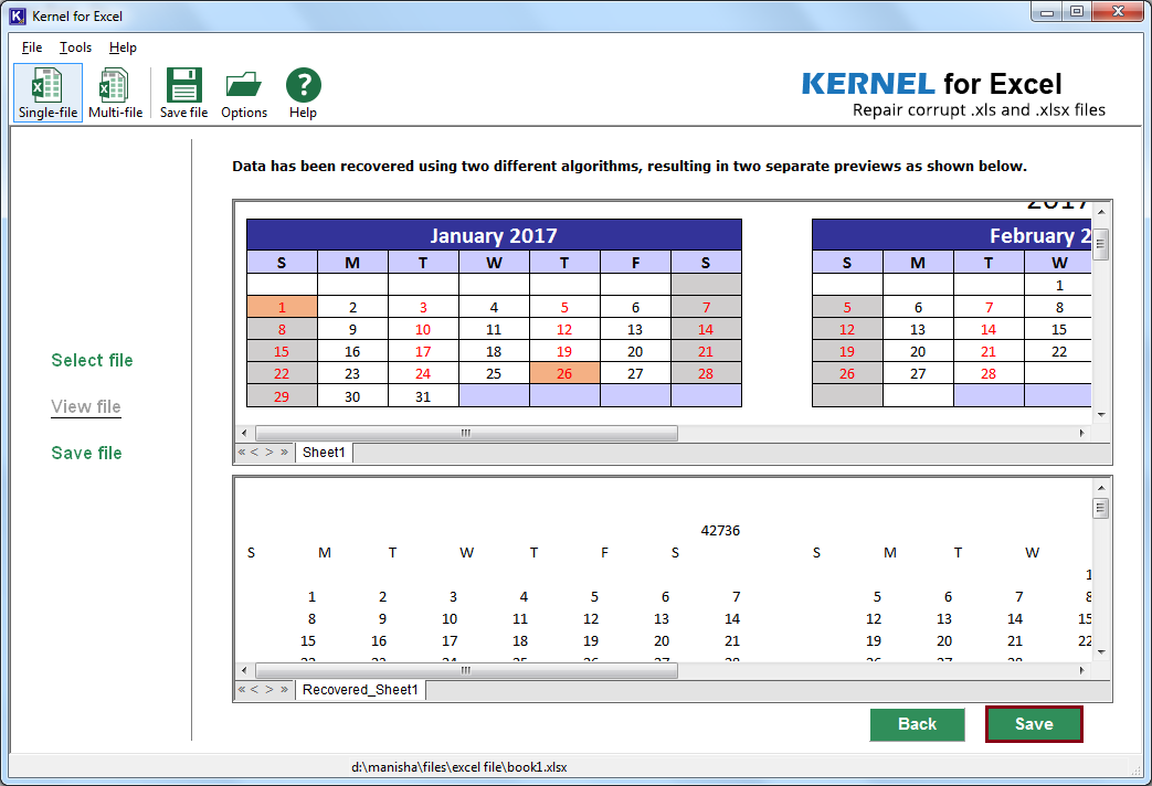
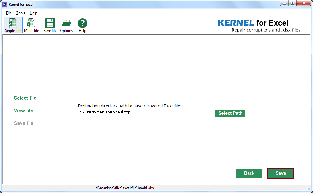
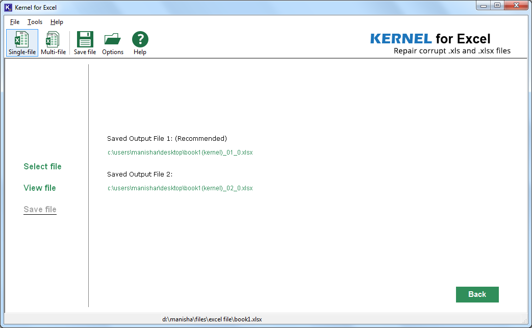
Kernel for Excel Repair is a powerful tool to recover your damaged Excel files after Excel errors. Embedded with powerful algorithms, this tool is a one-spot solution for all your Excel related issues. Moreover, you can download the trial version of the software free of cost. Here is the working of the tool.
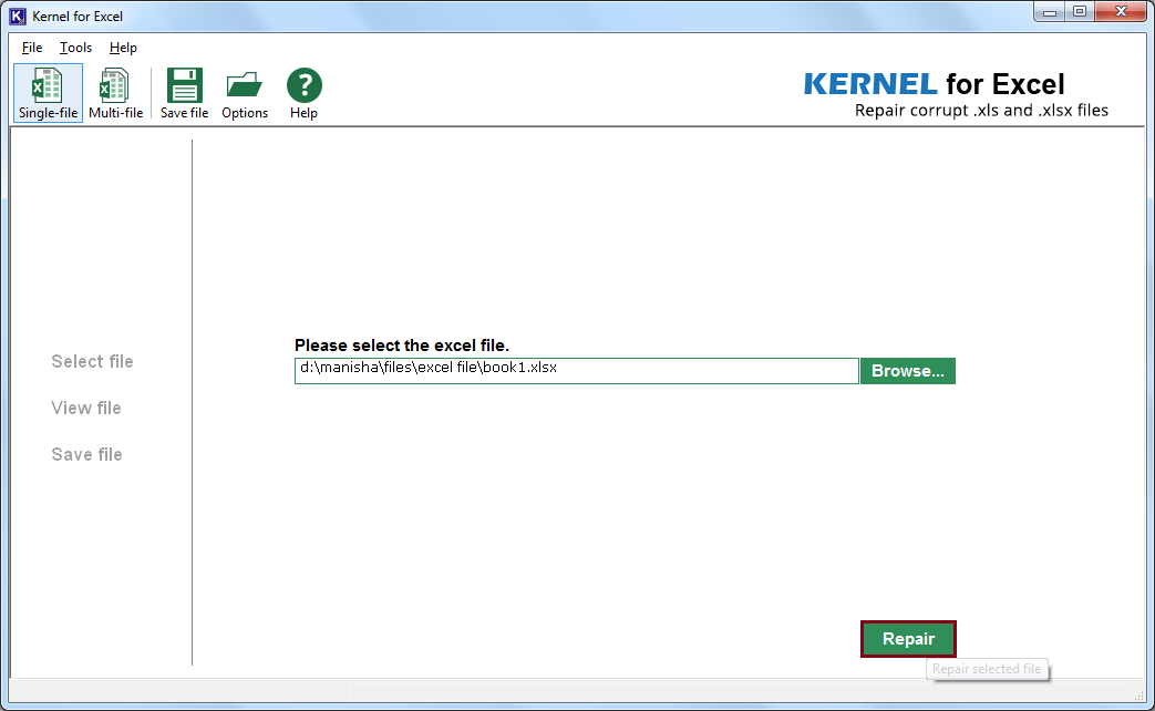
While you can fix #Value error by simple manual methods, some Excel errors are unpredictable and hard to fix. Moreover, there are various methods to recover corrupt excel files, but use of Kernel for Excel Repair tool is the best and the most recommended method to fix errors and recover damaged/corrupt Excel files.